Leaders in Lidar
- Visualizations by:
- Ryan Fitzgibbons
- Written by:
- Ryan Fitzgibbons
- Edited by:
- Ryan Fitzgibbons
- Scientific consulting by:
- Ryan Fitzgibbons,
- James Garvin, and
- Thomas A. Neumann
- Interviewees:
- Bryan Blair,
- David E. Smith,
- James Abshire,
- Jan McGarry,
- Jay Zwally,
- Ralph Dubayah,
- Scott Luthcke,
- Thomas A. Neumann, and
- Xiaoli Sun
- View full credits
Movies
- Series_Teaser_16-9.mp4 (1920x1080) [96.0 MB]
- Series_Teaser_16-9_prores.mov (1920x1080) [1.2 GB]
- Series_Teaser_16-9_prores.webm (1920x1080) [10.7 MB]
Captions
- SeriesTeaser16-9.en_US.srt [3.1 KB]
- SeriesTeaser16-9.en_US.vtt [2.9 KB]
Images
- LeadersLidarTeaser_thumb_print.jpg (1024x564) [274.9 KB]
- LeadersLidarTeaser_thumb.png (3326x1832) [10.3 MB]
- LeadersLidarTeaser_thumb_thm.png (80x40) [12.2 KB]
- LeadersLidarTeaser_thumb_searchweb.png (320x180) [131.7 KB]
Leaders in Lidar series teaser in standard format.
Music: "The Archives," Universal Production Music.
Complete transcript available.
Movies
- Ep1-1-6-23_prores.mov (1920x1080) [8.2 GB]
- Ep1-1-6-23.mp4 (1920x1080) [632.2 MB]
- Ep1-1-6-23_prores.webm (1920x1080) [67.0 MB]
Captions
- Ep1-v4.en_US.srt [13.3 KB]
- Ep1-v4.en_US.vtt [12.6 KB]
Images
- Lidar_Ch1_thumb_print.jpg (1024x575) [322.4 KB]
- Lidar_Ch1_thumb.png (1032x580) [1.4 MB]
- Lidar_Ch1_thumb_thm.png (80x40) [11.8 KB]
- Lidar_Ch1_thumb_searchweb.png (320x180) [136.8 KB]
Chapter 1: The Laser Is Better
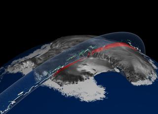
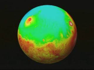
The scientists and engineers at Goddard Space Flight Center embark on a new technological and scientific journey, building and sending a laser altimeter to Mars with the MOLA-1 Instrument.
Music: "Fragment," "Chasing Lights," "Charming Noise," "Steady Pace," "The Cage," "Taking It All In," "The Archives," "Intriguing Coincidence," "Everyday Stories," Universal Production Music
Complete transcript available.
Video Descriptive Text available.
Note on footage used: 00:03-00:09 provided by pond5.
Movies
- Ep2-1-25-23b_prores.mov (1920x1080) [8.9 GB]
- Ep2-1-25-23b.mp4 (1920x1080) [685.4 MB]
- Ep2-1-25-23b_prores.webm (1920x1080) [73.0 MB]
Captions
- Ep2-v4.en_US.vtt [13.7 KB]
- Ep2-v4.en_US.srt [14.5 KB]
Images
- Lidar_Ch2_thumb.png (1008x570) [1.3 MB]
- Lidar_Ch2_thumb_print.jpg (1024x579) [315.4 KB]
- Lidar_Ch2_thumb_thm.png (80x40) [11.7 KB]
- Lidar_Ch2_thumb_searchweb.png (320x180) [136.3 KB]
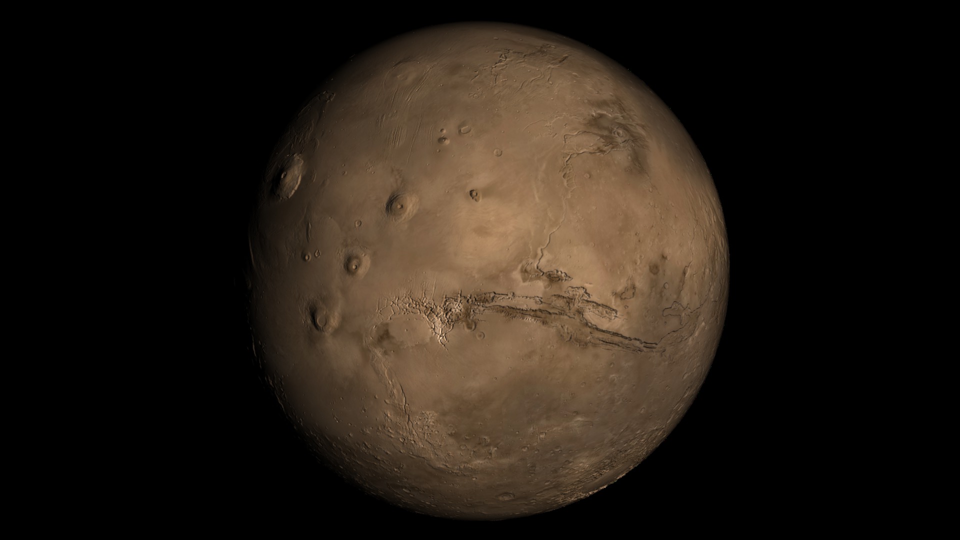
Chapter 2: Go Back to Mars
After the devastating loss of Mars Observer, the Goddard team mourns and regroups to build a second MOLA instrument for the Mars Global Surveyor mission. But before they send their laser altimeter to Mars, the team seizes an opportunity to test it on the Space Shuttle.
Music: "Unanswered Questions," "Chasing Lights," "Curious Occasion," "Time Ticking Away," "Have You Seen Annie," "Down to the Wire," "Man Versus Clock," "Everyday Stories." Universal Production Music.
Complete transcript available.
Video Descriptive Text available.
Movies
- Ep3-1-12-23.mp4 (1920x1080) [772.1 MB]
- Ep3-1-12-23_prores.mov (1920x1080) [10.1 GB]
- Ep3-1-12-23_prores.webm (1920x1080) [82.3 MB]
Captions
- Ep3-v3.en_US.vtt [15.3 KB]
- Ep3-v3.en_US.srt [16.1 KB]
Images
- Lidar_Ch3_thumb.png (1007x566) [1.4 MB]
- Lidar_Ch3_thumb_print.jpg (1024x575) [376.4 KB]
- Lidar_Ch3_thumb_thm.png (80x40) [11.9 KB]
- Lidar_Ch3_thumb_searchweb.png (320x180) [147.2 KB]
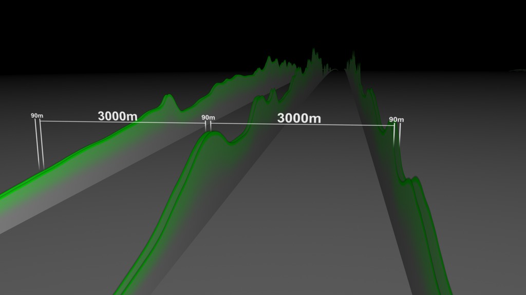
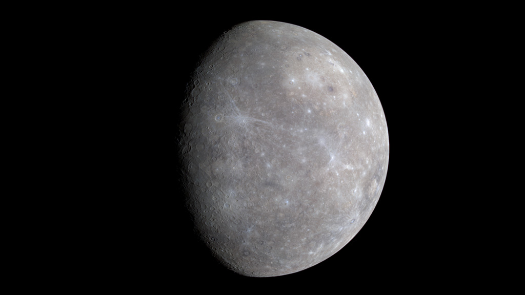
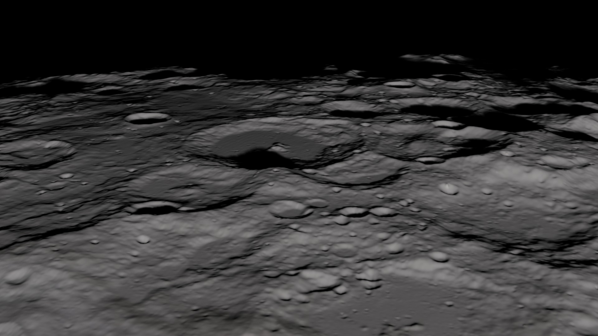
Chapter 3: Take the Next Steps
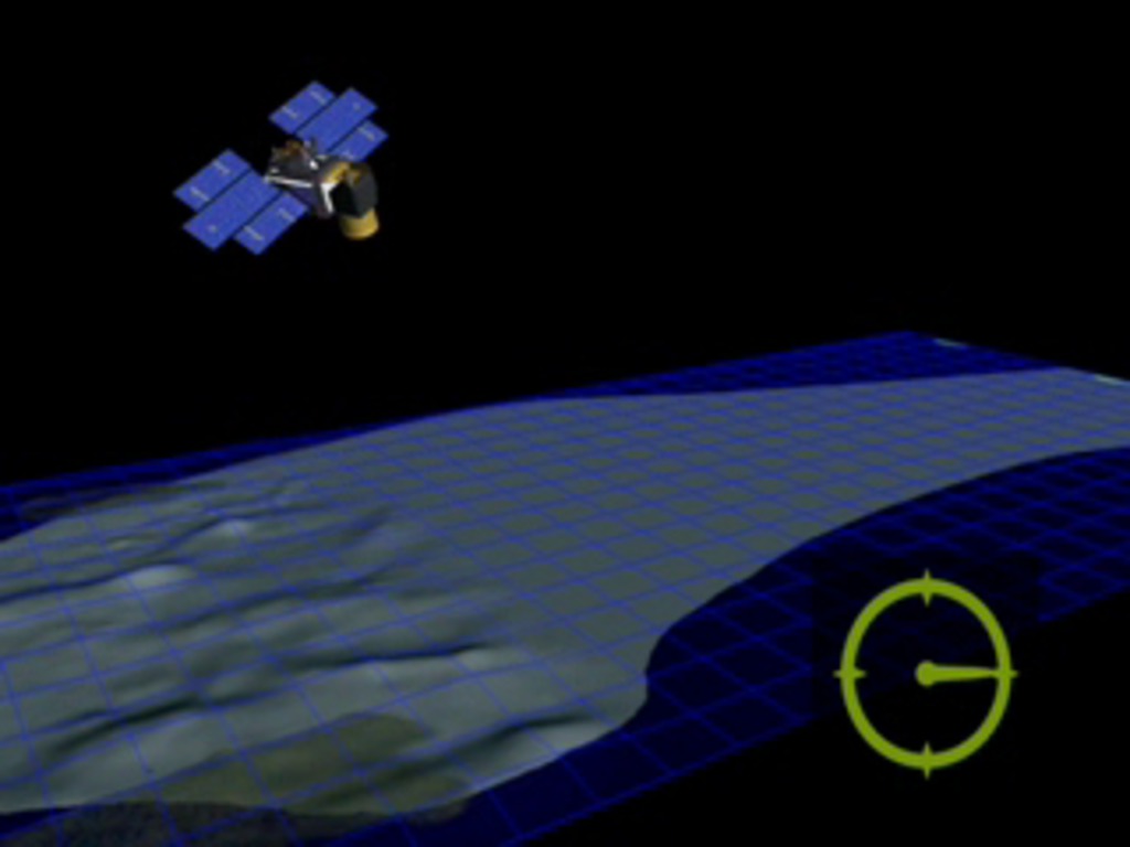
Riding on the success of MOLA, the Goddard team develops new lidar instruments for Earth, the Moon and Mercury. Each new instrument is a major leap forward in technology and scientific ambition and equally fraught with challenges.
Music: "Breakthrough Discovery," "Chasing Lights," "Prism Lights," "Ellipsis," "What Have We Done," "Resistor," "Starlight Andromeda," "Cascadia," "Everyday Stories," Universal Production Music.
Complete transcript available.
Video Descriptive Text available.
Note on footage used: 10:25 clip provided by pond5.
Movies
- Ep4-1-12-23.mp4 (1920x1080) [717.1 MB]
- Ep4-1-12-23.webm (1920x1080) [76.3 MB]
- Ep4-1-12-23_prores.mov (1920x1080) [9.6 GB]
- Ep4-1-12-23_prores.webm (1920x1080) [76.3 MB]
Captions
- Ep4-v4.en_US.vtt [14.6 KB]
- Ep4-v4.en_US.srt [15.4 KB]
Images
- Lidar_Ch4_thumb_print.jpg (1024x575) [342.1 KB]
- Lidar_Ch4_thumb.png (1031x579) [1.4 MB]
- Lidar_Ch4_thumb_thm.png (80x40) [11.8 KB]
- Lidar_Ch4_thumb_searchweb.png (320x180) [139.0 KB]
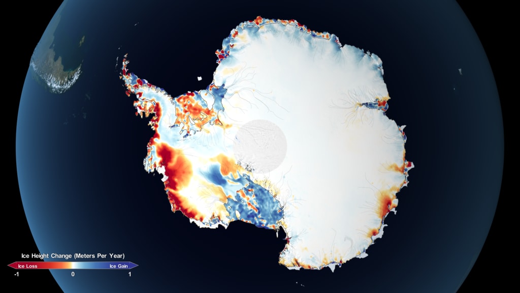
Chapter 4: All the Easy Missions Are Done
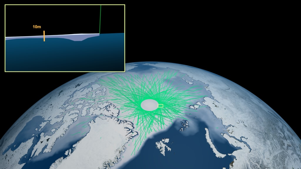
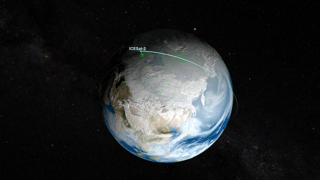
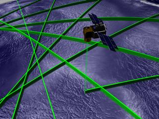
The Goddard team recounts the challenging paths that lead to the current lidar missions, the Global Ecosystems Dynamics Investigation (GEDI) and ICESat-2, which look to measure changes on our planet.
Music: "Quick Rhythmic Stabs," "Chasing Lights," "Little Magic," "In Broad Daylight," "Hidden between the Pages," "Down Is Not Out," "Curious by Nature," "Correlating Combination," "Everyday Stories," Universal Production Music.
Complete transcript available.
Video Descriptive Text available.
Movies
- SeriesTease_VERT.mp4 (1080x1920) [96.0 MB]
- SeriesTease_VERT.webm (1080x1920) [11.0 MB]
Captions
- SeriesTeaser_VERT.en_US.srt [3.1 KB]
- SeriesTeaser_VERT.en_US.vtt [2.9 KB]
Images
- seriestease_thumb_print.jpg (1024x1806) [584.4 KB]
- seriestease_thumb.png (402x709) [717.2 KB]
- seriestease_thumb_thm.png (80x40) [11.8 KB]
- seriestease_thumb_searchweb.png (320x180) [126.0 KB]
Series teaser for vertical Instagram Reels.
Music: "The Archives," Universal Production Music.
Complete transcript available.
Movies
- ThisIsAltimetry.mp4 (1080x1920) [70.2 MB]
- ThisIsAltimetry.webm (1080x1920) [8.2 MB]
Images
- ThisIsAltimeter-thumb_print.jpg (1024x1805) [266.5 KB]
- ThisIsAltimeter-thumb.png (447x788) [550.3 KB]
- ThisIsAltimeter-thumb_thm.png (80x40) [9.2 KB]
- ThisIsAltimeter-thumb_searchweb.png (320x180) [83.9 KB]
A supercut of scientists explaining how laser altimetry works. Formatted for vertical Instagram Reels.
Scientists and engineers eagerly await the first results of MOLA-2. Formatted for vertical Instagram Reels.
The team recall the challenges of building a much smaller laser altimeter to send to Mercury aboard the MESSENGER spacecraft. Formatted for vertical Instagram Reels.
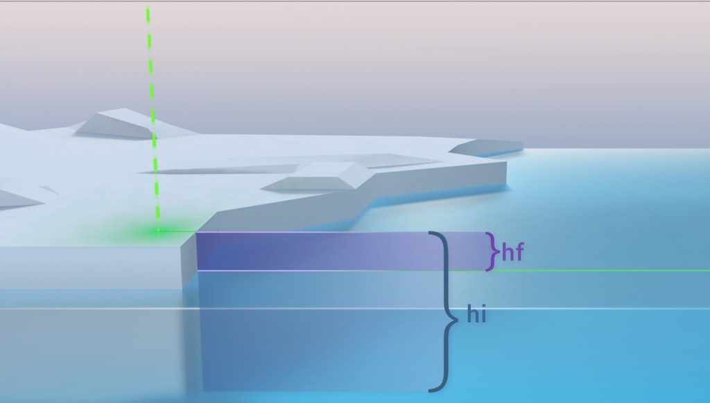
Engineer Scott Luthcke explains how geolocation allows for ICESat-2's precise ranging and measuring. Formatted for vertical Instagram Reels.
Credits
Please give credit for this item to:
NASA's Goddard Space Flight Center
Animators
- Ryan Fitzgibbons (KBRwyle) [Lead]
- Chris Meaney (KBRwyle)
- Susan Twardy (HTSI)
Visualizers
- Alex Kekesi (GST)
- Ernie Wright (USRA)
- Greg Shirah (NASA/GSFC)
- Kel Elkins (USRA)
Writer
- Ryan Fitzgibbons (KBRwyle) [Lead]
Editor
- Ryan Fitzgibbons (KBRwyle) [Lead]
Researcher
- Ryan Fitzgibbons (KBRwyle) [Lead]
Scientists
- James Garvin (NASA, Chief Scientist Goddard) [Lead]
- Thomas A. Neumann (NASA/GSFC) [Lead]
Interviewees
- Bryan Blair (NASA/GSFC) [Lead]
- David E. Smith (NASA/GSFC) [Lead]
- James Abshire (NASA/GSFC) [Lead]
- Jan McGarry (NASA/GSFC) [Lead]
- Jay Zwally (NASA/GSFC) [Lead]
- Ralph Dubayah (University of Maryland) [Lead]
- Scott Luthcke (NASA/GSFC) [Lead]
- Thomas A. Neumann (NASA/GSFC) [Lead]
- Xiaoli Sun (NASA/GSFC) [Lead]
- Jack L Bufton (GST)
- John F. Cavanaugh (NASA/GSFC)
- Joseph-Paul A. Swinski (NASA/GSFC)
Producer
- Ryan Fitzgibbons (KBRwyle) [Lead]
Narrator
- LK Ward (KBRwyle) [Lead]
Videographers
- Michael McClare (KBRwyle) [Lead]
- Rob Andreoli (AIMM) [Lead]
Project support
- James Garvin (NASA, Chief Scientist Goddard) [Lead]
- LK Ward (KBRwyle) [Lead]
- Thomas A. Neumann (NASA/GSFC) [Lead]
- David Lloyd Rabine (NASA/GSFC)
- Kathryn Mersmann (KBRwyle)
Technical support
- Aaron E. Lepsch (ADNET)
Series
This visualization can be found in the following series:Related pages
GEDI Forest Height
Oct. 29th, 2021
Read moreThis visualization depicts a global view of forest height data collected by the GEDI instrument aboard the International Space Station. Brown and dark green represent shorter vegetation. Bright green and white represent taller vegetation. This visualization uses data collected between April 2019 and April 2020. Height is exaggerated to depict variation at this scale.Coming soon to our YouTube channel. This is a closeup view of the GEDI forest height data collected for the west coast of the United States. Data is drawn on the globe over time, depicting how data coverage increases with each satellite pass. Brown and dark green represent shorter vegetation. Bright green and white represent taller vegetation. This visualization uses data collected between April 2018 and April 2019. Height is exaggerated to depict variation at this scale.Coming soon to our YouTube channel. Forest height color bar spanning 0m to 50m Forest height color bar spanning 0m to 75m Forest height color bar spanning 0m to 40m This visualization depicts a global view of forest height data collected by the GEDI instrument aboard the International Space Station. Brown and dark green represent shorter vegetation. Bright green and white represent taller vegetation. This visualization uses data collected between April 2018 and April 2019. Height is exaggerated to depict variation at this scale. This version has no on screen color bar. This is a closeup view of the GEDI forest height data collected for the west coast of the United States. Data is drawn on the globe over time, depicting how data coverage increases with each satellite pass. Brown and dark green represent shorter vegetation. Bright green and white represent taller vegetation. This visualization uses data collected between April 2018 and April 2019. Height is exaggerated to depict variation at this scale. This version has no on screen color bar. This is a closeup view of the GEDI forest height data collected over Florida. Data is drawn on the globe over time, depicting how data coverage increases with each satellite pass. Brown and dark green represent shorter vegetation. Bright green and white represent taller vegetation. This visualization uses data collected between April 2018 and April 2019. Height is exaggerated to depict variation at this scale. This is a closeup view of the GEDI forest height data collected over the Goddard Space Flight Center in Maryland. Data is drawn on the globe over time, depicting how data coverage increases with each satellite pass. Brown and dark green represent shorter vegetation. Bright green and white represent taller vegetation. This visualization uses data collected between April 2018 and April 2019. Height is exaggerated to depict variation at this scale. This is a closeup view of the GEDI forest height data collected over the Laurentides region around Quebec Canada. Data is drawn on the globe over time, depicting how data coverage increases with each satellite pass. Brown and dark green represent shorter vegetation. Bright green and white represent taller vegetation. This visualization uses data collected between April 2018 and April 2019. Height is exaggerated to depict variation at this scale. This is a closeup view of the GEDI forest height data collected over Senegal. Data is drawn on the globe over time, depicting how data coverage increases with each satellite pass. Brown and dark green represent shorter vegetation. Bright green and white represent taller vegetation. This visualization uses data collected between April 2018 and April 2019. Height is exaggerated to depict variation at this scale. This is a closeup view of the GEDI forest height data collected over Florida. Data is drawn on the globe over time, depicting how data coverage increases with each satellite pass. Brown and dark green represent shorter vegetation. Bright green and white represent taller vegetation. This visualization uses data collected between April 2018 and April 2019. Height is exaggerated to depict variation at this scale. This version has no on screen color bar. This is a closeup view of the GEDI forest height data collected over the Goddard Space Flight Center in Maryland. Data is drawn on the globe over time, depicting how data coverage increases with each satellite pass. Brown and dark green represent shorter vegetation. Bright green and white represent taller vegetation. This visualization uses data collected between April 2018 and April 2019. Height is exaggerated to depict variation at this scale. This version has no on screen color bar. This is a closeup view of the GEDI forest height data collected over the Laurentides region around Quebec Canada. Data is drawn on the globe over time, depicting how data coverage increases with each satellite pass. Brown and dark green represent shorter vegetation. Bright green and white represent taller vegetation. This visualization uses data collected between April 2018 and April 2019. Height is exaggerated to depict variation at this scale. This version has no on screen color bar. This is a closeup view of the GEDI forest height data collected over Senegal. Data is drawn on the globe over time, depicting how data coverage increases with each satellite pass. Brown and dark green represent shorter vegetation. Bright green and white represent taller vegetation. This visualization uses data collected between April 2018 and April 2019. Height is exaggerated to depict variation at this scale. This version has no on screen color bar. Still image depicting a global view of GEDI forest height data. Still image depicting a global view of GEDI forest height data. Still image depicting a global view of GEDI forest height data. Still image depicting a global view of GEDI forest height data. Still image depicting GEDI forest height data being collected over time. Camera is zoomed in on the west coast of the United States. Still image depicting GEDI forest height data being collected over time. Camera is zoomed in on the west coast of the United States. Still image depicting GEDI forest height data being collected over time. Camera is zoomed in on the west coast of the United States. Still image depicting GEDI forest height data being collected over time. Camera is zoomed in on the west coast of the United States. The Global Ecosystem Dynamics Investigation (GEDI) produces high resolution laser ranging observations of the 3D structure of the Earth. GEDI’s precise measurements of forest canopy height, canopy vertical structure, and surface elevation greatly advance our ability to characterize important carbon and water cycling processes, biodiversity, and habitat. GEDI’s data on surface structure are also of immense value for weather forecasting, forest management, glacier and snowpack monitoring, and the generation of more accurate digital elevation models. GEDI provides the missing piece – 3D structure – in NASA’s observational assets which enables us to better understand how the Earth behaves as a system, and guides the actions we can take to sustain critical resources. The GEDI instrument is a geodetic-class, light detection and ranging (lidar) laser system comprised of 3 lasers that produce 8 parallel tracks of observations. Each laser fires 242 times per second and illuminates a 25 m spot (a footprint) on the surface over which 3D structure is measured. Each footprint is separated by 60 m along track, with an across-track distance of about 600 m between each of the 8 tracks. GEDI expected to produce about 10 billion cloud-free observations during its nominal 24-month mission length.To learn more, visit the GEDI webpage Related pages
Land Ice Height Change Between ICESat and ICESat-2
April 30th, 2020
Read moreThis visualization depicts changes in Antarctic land ice thickness as measured by the ICESat (2003-2009) and ICESat-2 (2018-) satellites. The camera zooms into a region near the Kamb ice stream to compare ICESat and ICESat-2 beam tracks. The beam intersections are highlighted to explain how the data at these points are used to measure how land ice has changed over time. After exploring a few regions in detail, the camera moves out to a global view and an ocean temperature dataset is revealed. This visualization depicts changes in Greenland land ice thickness as measured by the ICESat (2003-2009) and ICESat-2 (2018-) satellites. The camera zooms into a region near the Zachariae Isstrom glacier to compare ICESat and ICESat-2 beam tracks. The beam intersections are highlighted to explain how the data at these points are used to measure how land ice has changed over time. This high resolution still image depicts changes in Antarctic land ice thickness as measured by the ICESat (2003-2009) and ICESat-2 (2018-) satellites. This high resolution still image depicts changes in Greenland land ice thickness as measured by the ICESat (2003-2009) and ICESat-2 (2018-) satellites. The future response of the Antarctic Ice Sheet to changes in climate is the single largest source of uncertainty in projections of sea level rise. If the ice sheet melted completely it would raise sea levels by 57 meters, a process that would unfold over millennia. One key to understanding how the ice sheet will respond in the future is to observe and analyze how the ice sheet has reacted to changes in climate over the past decades, where satellites observations are available. One key to understanding ice sheet change is to examine records of elevation change that show where the ice sheet is thinning and thickening due to changing environment. Recent analysis of incredibly precise surface elevations collected by NASA’s ICESat and ICESat-2 satellite laser altimeters reveals complex patters of ice sheet and ice shelf (floating extensions of the ice sheets) change that are the combined consequence of changes in melting by the ocean, changes in precipitation and, changes at the bed of the glacier where the ice sheet slides across the underlying bedrock. The researchers do this my finding locations where tracks of measured elevation intersect, measuring the change in elevation and correct for changes in the average density of the surface using models. Coherent regional patters of elevation change reveal the underlying mechanism responsible causing ice sheet change. One of the most striking features in the data is the Kamb Ice Stream that once flowed rapidly into the Ross Ice Shelf but that stopped flowing due to an increase friction (resistance to flow) likely caused by changes in the availability of liquid water at its base. Strong patters of thinning are visible all along the Amundsen Cost where ice shelves are rapidly thinning in response to increased melting by warm ocean waters. Melting of ice shelves do not directly contribute to changes in sea level, since they are already floating, but they do indirectly impact how fast the grounded ice is able to flow into the ocean. Ice shelves are located at the fronts of the glaciers and help to regulate how fast the ice flows into the ocean. As the ice shelves thin they become less able to hold back the inland ice, causing the grounded glaciers to accelerate and thin. In the East, broad patters of thickening reveal that the East Antarctic Ice Sheet is growing most likely in response to increases in precipitation relative to some unknown time in the past. The thickening is strongest along the coast of Dronning Maud Land where enhanced moisture transport has resulted in increased snowfall. Despite the diversity of gains and losses, losses in the West (208 cubic kilometers of water per year or Gt) greatly outpace Gains (90 Gt per year) in the east resulting in a total Antarctic mass change loss of 118 Gt per year. As the Greenland Ice Sheet responds to warming oceans and atmosphere it has become one of the largest contributors to sea level rise and will continue to be for the foreseeable future. Scientists are working to determine more precisely how much more ice will be lost and when that loss will occur. One key approach to doing this is to analyze changes in the ice sheets elevation over the past decades where satellite observations are available. By finding the intersection of elevation track measurements collected by NASA’s ICESat (2003-2009) and ICESat-2 (2018-) satellite laser altimeters, researchers are able to make very precise measurements of elevation change that can be converted to estimates of mass change after correcting for changes snow density using models. The combination of long time-span between measurements and the high accuracy of NASA’s satellite laser altimeters allows the researchers to make highly detailed maps of mass change that provide insights into the mechanism behind the ice sheets rapid rate of loss. Thinning can be seen around the periphery of the ice sheet where elevations are closest to sea level and rates of surface melting are highest. This pattern is punctuated by localized areas of extreme thinning where large glaciers come into contact with warm ocean waters. Unlike the uniform pattern of low-elevation thinning that is being driven by increased melting due to warmer summer air temperatures, these concentrated areas of thinning occur where outlet glacier have sped up. These glaciers have sped up in response to some combination of retreating ice front position, changes in the slipperiness at the bed of the glacier due to changes in liquid water at the ice-rock interface and due to change in the rate frontal melting due to an increase in the heat content of the ocean waters that come into contact with the glacier front. Juxtaposed on the pattern of rapid thinning along the periphery of the ice sheet is a broad pattern of thickening in the high-elevation interior of the ice sheet. This pattern of thickening suggests that increases in snowfall, relative to sometime in the past, are partly compensating for increased losses due to enhanced melt and accelerated glacier flow. Overall low-elevation losses greatly outpace high-elevation gains resulting in 3200 cubic kilometers of water (Gt) being lost from the ice sheets and entering the oceans, raising global mean sea level by 8.9 mm. Related pages
Measuring Sea Ice Thickness with ICESat-2
Sept. 5th, 2019
Read moreThis visualization depicts sea ice thickness in the Arctic Ocean as measured by ICESat-2 over the course of several months. The visualization begins with a global view of the north pole as individual tracks are drawn over time representing each time the satellite passes overhead and collects sea ice data. A closeup view of one track is revealed, showing how the ICESat-2 laser can measure ice freeboard (height above sea level), which can be used to calculate total ice thickness. The visualization concludes by showing monthly average of sea ice thickness from November 2018 to March 2019. ICESat-2 tracks over the Arctic Ocean spanning from November 2018 to March 2019. A view of the Arctic Ocean with monthly average sea ice thickness spanning November 2018 to March 2019. Low values are depicted in light blue, and higher values (5 meters) are depicted in magenta. Close up view of a single ICESat-2 track. The light grey section of the track represented ice freeboard (height above sea level) and the darker grey represents sea ice below the ocean surface. A 10m orange line is shown for scale. One of the big challenges in polar science is measuring the thickness of the floating sea ice that blankets the Arctic and Southern Oceans. Newly formed sea ice might be only a few inches thick, whereas sea ice that survives several winter seasons can grow to several feet in thickness (over ten feet in some places). Sea ice thickness is typically estimated by first measuring sea ice freeboard - how much of the floating ice can be observed above sea level. Sea ice floats slightly above sea level because it is less dense than water. NASA’s ICESat-2 satellite measures the Earth’s surface height by firing green laser pulses towards Earth and timing how long it takes for those laser pulses to reflect back to the satellite. Ice freeboard is calculated by differencing the heights of the ice surface and areas of open water next to the ice. Additional information including the depth and density of the snow layer on top of the ice is needed to convert this freeboard measurement to sea ice thickness. New state-of-the-art snow accumulation models have been developed to provide this extra data in preparation for the launch of ICESat-2. The very high precision of the ICESat-2 laser has enabled us for to measure the thickness of very thin sea ice for the first time. As the Arctic warms rapidly it is becoming increasingly dominated by a younger and thinner ice cover, making these new measurements extremely invaluable for understanding our changing polar regions. Related pages
GEDI Media Resources
Oct. 9th, 2018
Read moreAnimation of the Global Ecosystem Dynamics Investigation (GEDI) instrument, as installed on the ISS, showing the three lasers, which are split into 4 beams that alternate to give 8 footprints across a 4.2 km swath when they hit the ground. The animation ends with an illustration of a laser pulse interacting with a multi-level forest canopy and the ground, culminating in an example of the waveform that is generated by the return of reflected photons to GEDI. B-roll footage of the Global Ecosystem Dynamics Investigation (GEDI) instrument being built and tested at NASA's Goddard Space Flight Center in 2018.GEDI is a full-waveform lidar instrument that makes detailed measurements of the 3D structure of the Earth’s surface. Lidar is an active remote sensing technology (the laser version of radar) which uses pulses of laser light to measure 3D structure. The light is reflected by the ground, vegetation and any clouds and is then collected by GEDI’s telescope. These photons are sent to detectors, recording time of arrival in 1 ns (15 cm) intervals. Time is converted to distance by multiplying by the speed of light. GEDI contains three Nd:YAG lasers, emitting 1064 nm light. These pulse 242 times per second with a power of 10 mJ, firing short pulses of light (14 ns long) down towards the Earth’s surface with a beam divergence of 56 mrad, resulting in footprints averaging 25 m in diameter.Two of the lasers are full power, and one is split into two beams, producing a total of four beams. Beam Dithering Units (BDUs) rapidly change the deflection of the outgoing laser beams by 1.5 mrad, shifting them by 600 m on the ground. This produces eight ground tracks; four power and four cover tracks. Footprints are separated by 60 m along-track and 600 m across track. The Global Ecosystem Dynamics Investigation (GEDI) uses laser pulses to give a view of the 3D structure of the Earth. GEDI’s precise measurements of the height and vertical structure of forest canopy, along with the surface elevation, will greatly advance our ability to characterize important carbon and water cycling processes, biodiversity, and habitat. The mission is led by the University of Maryland, College Park, and the instrument was built and tested at NASA's Goddard Space Flight Center.GEDI observes nearly all tropical and temperate forests using a self-contained laser altimeter on the International Space Station. GEDI has the highest resolution and densest sampling of any lidar ever put in orbit. This has required a number of innovative technologies to be developed at NASA Goddard.GEDI has three lasers that produce 8 parallel tracks of observations. Each laser fires 242 times per second and illuminates a 25-meter footprint on the surface over which 3D structure is measured. Each footprint is separated by 60 meters along the track, with an across-track distance of about 600 m between each of the 8 tracks. GEDI is expected to produce about 10 billion cloud-free observations during its nominal 24-month mission length.With these observations, GEDI will provide answers to how deforestation has contributed to atmospheric CO2 concentrations, how much carbon forests will absorb in the future, and how habitat degradation will affect global biodiversity. This data is of immense value for forest and water resource management, carbon cycle science, and weather prediction.For more information about GEDI: https://gedi.umd.edu Related pages
ICESat-2 Measures Sea Ice Thickness
Aug. 22nd, 2018
Read moreAnimation showing how ICESat-2 will measure the height of sea ice freeboard (hf) – the portion of sea ice floating above the water – to estimate sea ice thickness (hi). ICESat-2 will measure heights or elevations. In order to derive sea ice thickness from those measurements, it will compare the height of the ice with the height of the adjacent open water. The difference is height is the portion of the ice that is above the sea level, called freeboard. Because roughly 1/10 of the ice floe is above water we can calculate its thickness. Very often the only open water nearby is from cracks in the ice (leads) that open and close quickly as the ice drifts about in the polar oceans pushed by ocean currents and winds. Related pages
ICESat-2 Orbit
Nov. 3rd, 2017
Read moreICESat-2 orbiting Earth: starting with global view building up ground track, then riding the satellite view, then back to a global view with full ground track ICESat-2 orbit with ground track (short version) ICESat-2 is a spacecraft designed to accurately measure land and ice elevations on Earth. By comparing observations from different times, scientists will be able to study changes in elevations. ICESat-2 will be in a polar orbit which will provide high coverage near the poles where ice elevations are changing relatively quickly. This visualization shows ICESat-2's polar orbit from afar, then closer up. As we get close to the satellite, the 3 pairs of ICESat-2's ATLAS lidar laser beams begin to resolve. A ground track shows ICESat-2's global coverage which repeats about once every 90 days.The ATLAS lidar on ICESat-2 uses 3 pairs of laser beams to measure the earth’s elevation and elevation change. As a global mission, ICESat-2 will collect data over the entire globe, however the ATLAS instrument is optimized to measure land ice and sea ice elevation in the polar regions.For more information on ICESat-2 click here. Related pages
ICESat-2 Measurements Over Antarctica (prelaunch)
Nov. 9th, 2016
Read moreICESat-2 has 3 pairs of lasers that will measure the heights of ice and snow at very high resolution The ATLAS lidar on ICESat-2 uses 6 laser beams to measure the earth’s elevation and elevation change. As a global mission, ICESat-2 will collect data over the entire globe, however the ATLAS instrument is optimized to measure land ice and sea ice elevation in the polar regions. ICESat-2 reports elevations with respect to a reference surface, called an ellipsoid. In this measurement system, shared by GPS devices, an elevation of zero meters indicates the notional sea level, although tides, wind, and waves can make the actual sea level either greater than or less than zero. The Antarctic ice sheet, shown here, ranges up to 4000m above sea level. Over the course of 91 days, ATLAS will generate 1387 ground tracks across Antarctica for each of it’s 6 beams. Related pages
Untitled
May 12th, 2015
Read moreAfter four years of exploring Mercury from orbit, NASA’s MESSENGER mission comes to an end. Mercury's surface is heavily cratered like our moon. This elevation map shows high terrain in white, and low-lying areas in purple. Central peaks within Mercury's Abedin crater surround a curious depression (center), which may be volcanic in origin. MESSENGER found temperatures in sunlit areas (red) and shadowed regions (blue, purple) at Mercury's north pole could differ by more than 1,000°F. The colors in this image represent different types of geologic material seen in one of Mercury's impact basins. Mercury is colored in the image on the right to show the diverse array of minerals on its surface. Related pages
Mars Roll
Dec. 27th, 2011
Read moreAnimation that rolls Mars around to show all the major features of the Martian topography. This animation begins with a hemispherical view of Olympus Mons and Valles Marineris and then rolls around to reveal the Martian South Pole. While traversing Northward, we pass Hellas Basin and end up looking down up the Martian North Pole. Print resolution image of Mars showing a partly shadowed Olympus Mons toward the upper left of the image. The row of 3 volcanoes that form the base of a triangle in relationship to Olympus Mons are (from top to bottom): Ascraeus Mons, Pavonis Mons, and Arsia Mons. Valles Marineris can also be seen. It's the giant valley that slashes equatorially across the Martian landscape to the right of the volcanoes. Print resolution nadir view of the Martian South Pole. Print resolution image of Mars. Hellas Basin can be seen in the lower right portion of the image. Print resolution image of Mars slightly tilted to show the Martian North Pole. Print resolution nadir view of the Martian North Pole. A redux of entry #2455 using MGS/MOLA data for the Martian topography and MGS/MOC for the Martian surface color. The animation rolls Mars to show major features of the Martian topography. Major features depicted include: Olympus Mons, Valles Marineris, Hellas Basin, and the Martian North and South Poles. Related pages
LRO/LOLA Lunar South Pole Flyover
March 14th, 2010
Read moreThis animation flys around the moon's south pole. Some of the craters on this tour are: Amundsen, Cabeus, Haworth, Faustini, Malapert, Laveran, Scott, Shackleton, Shoemaker, and Wiechert Sample animation using the match-frame rendered crater annotations from animation #3633 as an overlay to annotate the craters in this flyover. Print resolution still of the moon. Print resolution still of our simulated approach to the lunar surface. Print resolution still over the lunar south pole. Craters depicted in this image are Laveran, Wiechert, Amundsen, Faustini, Shackleton, Shoemaker, Scott, and Haworth. Print resolution still of the lunar south pole. Top down view of the south pole region. The Lunar Reconnaissance Oribiter (LRO) was launched on June 18, 2009. Its mission is to map the moon's surface, find safe landing sites, locate potential resources, characterize the radiation environment, and demonstrate new technology. One of the instruments on board is the Lunar Orbiter Laser Altimeter (LOLA) which measures landing site slopes, lunar surface roughness, and has begun generation of a high resolution 3D map of the Moon.This visualization uses Clementine data for the global view of the moon, but then transitions to using only LRO/LOLA DEM with a neutral gray texture when flying around the lunar south pole. The DEM by itself creates an amazingly realistic view of the lunar southpole. As better maps are created from the other instruments aboard LRO, an even clearer picture of the moon will emerge.Please note that this visualization is match-frame rendered to The Moon's South Pole in 3D via LRO/LOLA First Light Data (#3633). Related pages
The Moon's South Pole in 3D via LRO/LOLA First Light Data
Sept. 15th, 2009
Read moreThis animation shows some of the first results of the LRO/LOLA instrument with labels over several craters. As the virtual camera flies around the lunar south pole we not only get an indication of the moon's mysterious topography at this pole, but also a sense that this mission has just begun. This animation shows some of the first results of the LRO/LOLA instrument without any labels. Colorbar for lunar elevations. Print resolution still of the moon with some early swaths of LOLA data. Print resolution still of the LRO/LOLA data swaths as they are laid out on the lunar surface. Please note that for aesthetic purposes the swath widths are shown wider than actual. The actual width of a swath is approximately 65 meters across. Print resolution still over the lunar south pole. Craters depicted in this image are Scott, Amundsen, Faustini, Shoemaker, Haworth, Malapert, Shackleton, and Wiechert. Print resolution still of the lunar south pole. Top down view of the south pole region. The Lunar Reconnaissance Oribiter (LRO) was launched on June 18, 2009. Its mission is to map the moon's surface, find safe landing sites, locate potential resources, characterize the radiation environment, and demonstrate new technology. One of the instruments on board is the Lunar Orbiter Laser Altimeter (LOLA) which measures landing site slopes, lunar surface roughness, and has begun generation of a high resolution 3D map of the Moon. The animation depicted here is the beginning of LOLA's mapping project and shows the lunar south pole through digital elevation map data collected by the LOLA instrument during the spacecraft commissioning phase. During the commissioning phase, LRO was in a highly elliptical orbit coming closer to the lunar south pole than the north pole. Furthermore, since LOLA uses laser pulses to measure the surface, the accuracy of its measurements are greatly affected by the instrument's distance to the surface. This is why there is virtually no data of the lunar north pole, and much better coverage of the south pole. The topographic data shown here is currently processed to show at approximately 30 meters per pixel.The colors in this animation depict the relative heights of the lunar surface with respect to the surface mean. Warm colors (brown, red, magenta, and tan) indicate areas above the mean. Cooler colors (green, cyan, blue, and violet) are areas below the mean. Related pages
ICESat Lithograph
Sept. 3rd, 2004
Read moreA view of Antarctica showing ice sheet elevation and cloud data from ICESat This still image was generated to be printed as a lithograph for public distribution. [from the litho:] This image illustrates ice sheet elevation and cloud data from ICESat's Geoscience Laser Altimeter System (GLAS) on its first day of operation, February 20, 2003. On that day, the instrument collected a 1064 nm wavelength profile across Antarctica: the lower West Antarctic Ice Sheet in the foreground is separated from the higher East Antarctic Ice Sheet in the background by the steep TransAntarctic Mountains. The elevation profile (in red) is depicted relative to the Earthandapos;s standard ellipsoid with 50x vertical exaggeration. Data collected across floating sea ice and open water of the adjacent Southern Ocean cannot be shown at this scale. Clouds of various thicknesses are indicated by colors changing progressively from light blue (thin clouds) to white (opaque layers). Note that the laser cannot penetrate the thickest clouds causing gaps in the elevation profile below. The RADARSAT (Canadian Space Agency) mosaic is used to illustrate the Antarctic continent. Related pages
ICESat Data Accumulation Animation
Feb. 9th, 2004
Read moreThis is the standard definition version MPEG of the ICESat Data Accumulation Animation. Accumulating Data: Glas Builds Its Facts One Point at a Time - The technology behind GLAS is called lidar. Lidar is a distance measuring system similar to radar, except that instead of radio waves it uses pulses of laser light for range finding. The name is a contraction based on the words light and radar: Light Detection And Ranging. A lidar system determines precise distances by measuring the amount of time necessary for a pulse of light to leave an emitter, hit a target, and return. In this case, distance measurements helped researchers determine changes in ice thickness, vegetation, cloud thickness, and much more. Related pages
ICESat First Light Release: Following ICESat
May 15th, 2003
Read moreAnimation showing ICESat collecting elevation data ICESat collecting elevation data Video slate image reads "ICESat First Light: Following ICESat". In this visualization we ride along with the ICESat spacecraft as its laser measures detailed changes in surface topography. This was produced in support of the ICESat first light release. Related pages
A Rotating False Color View of the Martian South Pole from MOLA
Nov. 22nd, 1999
Read moreA rotating view of the Martian south pole using MOLA topography data The visible Martian south polar cap appears outlined in black, but the accompanying false color data shows the topographically inferred extent of the polar layered terrain. False color image of Mars from MOLA data. Here the color scale shows the darkest blues as roughly 8 km below the mean equatorial height, while reds indicate elevations up to 5 km above the mean equatorial height. MOLA data of Martian topography highlighting the differences in elevation between the Hellas Impact Basin and surrounding terrain. The deepest point in Hellas is roughly 8200 meters below the equatorial mean. This is one of a series of visualizations showing false-colored renderings of the Martian topography measured by MOLA in the vicinity of the Mars Polar Lander landing site. Blue tones represent elevations of less than 2 kilometers, while reddish tones are greater than about 2.8 kilometers, relative to the mean equatorial height of Mars. The elevation of the landing site is about 2.4 km, midway into the polar layered terrain. The 400 meters (1/4 mile) resolution of the MOLA data gives a smoothed but vertically exaggerated view of the topography. At this scale it is impossible to ascertain the actual roughness at the lander's destination, forcing project directors to make their best guesses based on available data. For More InformationSee [http://svs.gsfc.nasa.gov/stories/MOLA_south_pole/index.html](http://svs.gsfc.nasa.gov/stories/MOLA_south_pole/index.html) Related pages
Supporting Media for MOLA release
July 10th, 1990
Read moreHow the spacecraft made the gravity map. Animation by Studio 13. Evidence of global magnetic field on Mars collected by Mars Global Surveyor (MGS). Animation by Studio 13. Dramatic asymmetry in structure between north and south. North took longer to cool suggests that there may have once been a northernmartian ocean. Animation by Studio 13. How MGS made the gravity map. Animation by Studio 13. Animation of how MOLA takes elevation readings. Animation by Studio 13. How the spacecraft made the gravity map. Animation by Studio 13. Evidence of global magnetic field on Mars collected by Mars Global Surveyor (MGS). Animation by Studio 13. Dramatic asymmetry in structure between north and south. North took longer to cool suggests that there may have once been a northern martian ocean. Animation by Studio 13. How MGS made the gravity map. Animation by Studio 13. How Mars Orbiter uses its laser altimeter to collect elevation data. Animation by Studio 13. For More InformationSee [http://svs.gsfc.nasa.gov/stories/MOLA/index.html](http://svs.gsfc.nasa.gov/stories/MOLA/index.html) Related pages