How NASA Satellites Help Model the Future of Climate
Music: "Connections Established," "Data Visions," Universal Production Music
Complete transcript available.
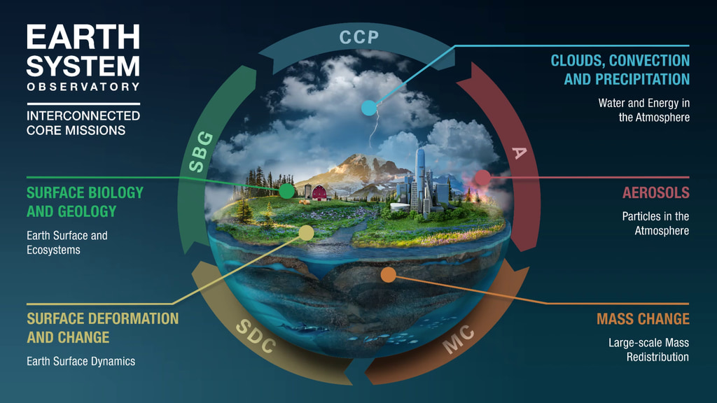
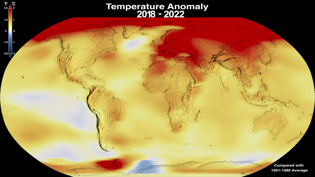
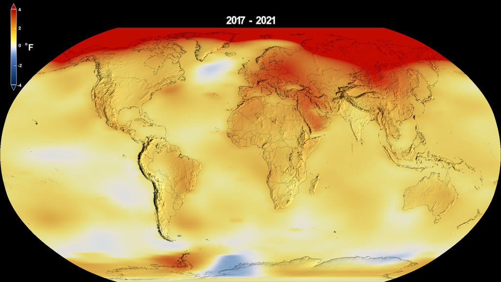
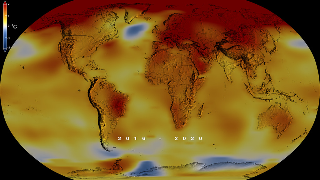
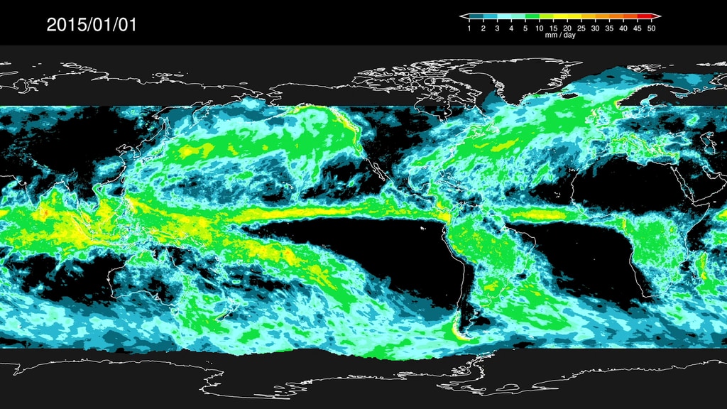
Continuing key observations of the Earth is really important to see how our atmosphere, land and oceans are changing over time. A long term record, combined with cutting edge observations from the new NASA Earth System Observatory, will continue to push boundaries to better understand our ever changing Earth.
Credits
Please give credit for this item to:
NASA's Goddard Space Flight Center
-
Producer
- Ryan Fitzgibbons (KBR Wyle Services, LLC)
-
Narrator
- LK Ward (KBR Wyle Services, LLC)
-
Scientists
- Kate Marvel (NASA/GSFC GISS)
- Dalia B Kirschbaum (NASA/GSFC)
- Greg S Elsaesser (Columbia University)
-
Writer
- Ryan Fitzgibbons (KBR Wyle Services, LLC)
-
Editor
- Ryan Fitzgibbons (KBR Wyle Services, LLC)
-
Interviewee
- Min-Jeong Kim (Morgan State University)
-
Animator
- Ryan Fitzgibbons (KBR Wyle Services, LLC)
Release date
This page was originally published on Tuesday, August 24, 2021.
This page was last updated on Wednesday, May 3, 2023 at 1:43 PM EDT.
Missions
This visualization is related to the following missions:Series
This visualization can be found in the following series:Related
- ID: 14364
 Produced Video
 - ID: 4920
 Visualization
 - ID: 13567
![Music: Favor by Victor Maitre [SACEM]Complete transcript available.](/vis/a010000/a013500/a013567/GMAOThumb.jpg) Produced Video
Produced Video
Sources
- ID: 5060
 Visualization
 - ID: 4964
 Visualization
 - ID: 12772
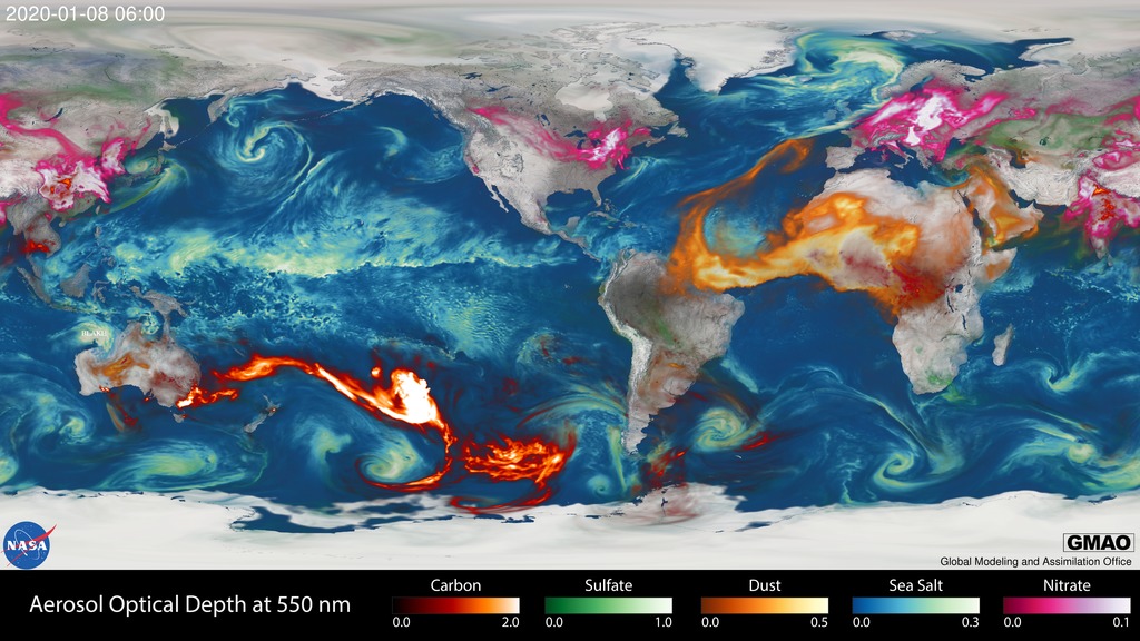
![Tracking aerosols over land and water from August 1 to November 1, 2017. Hurricanes and tropical storms are obvious from the large amounts of sea salt particles caught up in their swirling winds. The dust blowing off the Sahara, however, gets caught by water droplets and is rained out of the storm system. Smoke from the massive fires in the Pacific Northwest region of North America are blown across the Atlantic to the UK and Europe. This visualization is a result of combining NASA satellite data with sophisticated mathematical models that describe the underlying physical processes.Music: Elapsing Time by Christian Telford [ASCAP], Robert Anthony Navarro [ASCAP]Complete transcript available.Watch this video on the NASA Goddard YouTube channel.](/vis/a010000/a012700/a012772/12772_hurricanes_and_aerosols_1080p_youtube_1080.00001_print.jpg) Produced Video
Produced Video - ID: 4882
 Visualization
 - ID: 4799
 Visualization
 - ID: 4837
 Visualization
 - ID: 31139
 Hyperwall Visual
 - ID: 4796
 Visualization
 - ID: 4801
 Visualization
 - ID: 4802

- ID: 4815
 Visualization
 - ID: 4818
 Visualization
 - ID: 4819
 Visualization
 - ID: 4806
 Visualization
 - ID: 31100
 Hyperwall Visual
 - ID: 4789
 Visualization
 - ID: 4754
- ID: 13347
 Produced Video
 - ID: 4760
 Visualization
 - ID: 4759
 Visualization
 - ID: 4654
- ID: 4514
 Visualization
 - ID: 30590
 Hyperwall Visual