NASA Laser and ESA Radar Sync Up for Sea Ice
One of the big challenges in polar science is measuring the thickness of the floating sea ice that blankets the Arctic and Southern Oceans. Newly formed sea ice might be only a few inches thick, whereas sea ice that survives several winter seasons can grow to several feet in thickness (over ten feet in some places).
Sea ice thickness is typically estimated by first measuring sea ice freeboard - how much of the floating ice can be observed above sea level. Sea ice floats slightly above sea level because it is less dense than water. An additional complexity is that snow fall on sea ice pushes the floating ice downward and has a lower density than the sea ice. In order to estimate the sea ice thickness, some accommodation for the overlying snow must be made.
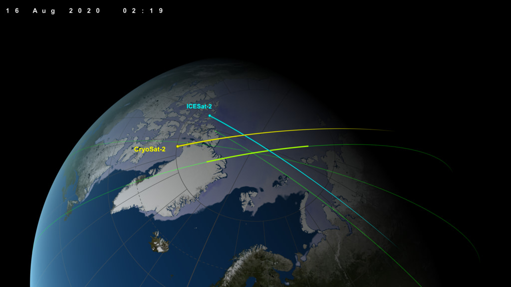
NASA’s ICESat-2 satellite measures the Earth’s surface height by firing green laser pulses towards Earth and timing how long it takes for those laser pulses to reflect back to the satellite. The laser light reflects off the top of the snow layer on top of the sea ice. In contrast, the European Space Agency’s CryoSat-2 mission uses radar waves to measure height. These radar waves penetrate the overlying snow and are reflected off the sea ice, rather than the overlying snow.
In July 2020, ESA elected to slightly perturb the orbit of CryoSat-2 to increase the overlap with ICESat-2. Given their different orbit altitudes, the result is a ~3000km stretch of sea ice that is measured by both ICESat-2 and CryoSat-2. By combining data from these two sensors, scientists can measure the snow layer thickness, and produce substantially improved sea ice thickness estimates.
Credits
Please give credit for this item to:
NASA's Goddard Space Flight Center
-
Producer
- Ryan Fitzgibbons (USRA)
-
Scientists
- Thomas A. Neumann (NASA/GSFC)
- Nathan T. Kurtz (NASA/GSFC)
-
Visualizer
- Kel Elkins (USRA)
-
Writer
- Kate Ramsayer (Telophase)
Release date
This page was originally published on Thursday, July 16, 2020.
This page was last updated on Wednesday, May 3, 2023 at 1:44 PM EDT.
Missions
This visualization is related to the following missions:Series
This visualization can be found in the following series:Sources
- ID: 4841
 Visualization