Earth from Orbit 2019: How NASA Satellites #PictureEarth
Music: After the Sun by Andrew Michael Britton [PRS], David Stephen Goldsmith [PRS], Andrew Skeet [PRS]
Complete transcript available.
This Earth Day, NASA invites you to share how you #PictureEarth. For inspiration, NASA collected some of the best and most inconic satellite images and data visualizations capture over the last year. NASA's space-based view of our planet, and the way it's changing, helps humans understand Earth better.
Image Sources:
International Space Station: Clouds and Continents
https://eol.jsc.nasa.gov/BeyondThePhotography/CrewEarthObservationsVideos/
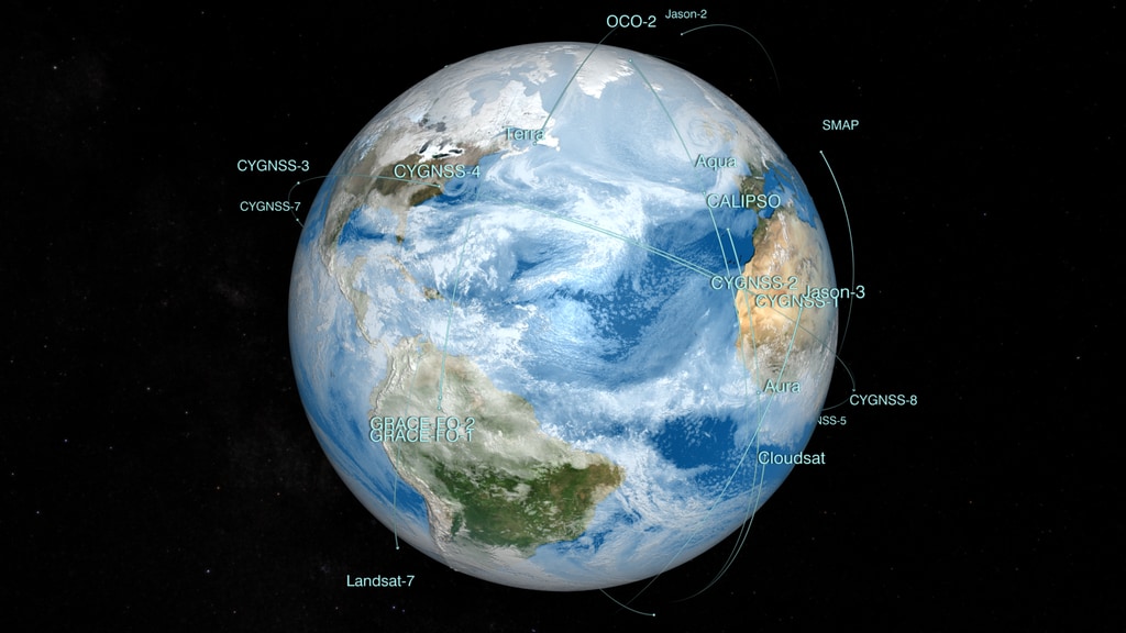
Earth Observing Fleet (June 2018)
https://svs.gsfc.nasa.gov/4662
A Clear Spring View of the Great Lakes
https://earthobservatory.nasa.gov/images/144747/a-clear-spring-view-of-the-great-lakes
A Spacecraft’s Journey to the Space Station
https://earthobservatory.nasa.gov/images/144408/a-spacecrafts-journey-to-the-space-station
Etna Awakens on its Side
https://earthobservatory.nasa.gov/images/144493/etna-awakens-on-its-side
Urban Growth in Las Vegas
https://svs.gsfc.nasa.gov/30215
Pinwheel Squares in Bolivia
https://earthobservatory.nasa.gov/images/144717/pinwheel-squares-in-bolivia
Aquaculture in China
https://earthobservatory.nasa.gov/images/144624/seaweed-and-fish-world
Growth of Medina, Saudi Arabia
https://earthobservatory.nasa.gov/images/144471/living-on-lava
Phytoplankton Bloom in the Baltic Sea
https://earthobservatory.nasa.gov/images/144643/jupiter-or-earth
Typhoon Mangkhut
https://earthobservatory.nasa.gov/images/92749/mangkhut-bearing-down-on-the-philippines
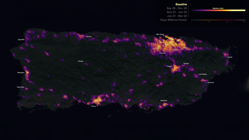
Hurricane Maria and Disaster Recovery in Puerto Rico
https://svs.gsfc.nasa.gov/4658
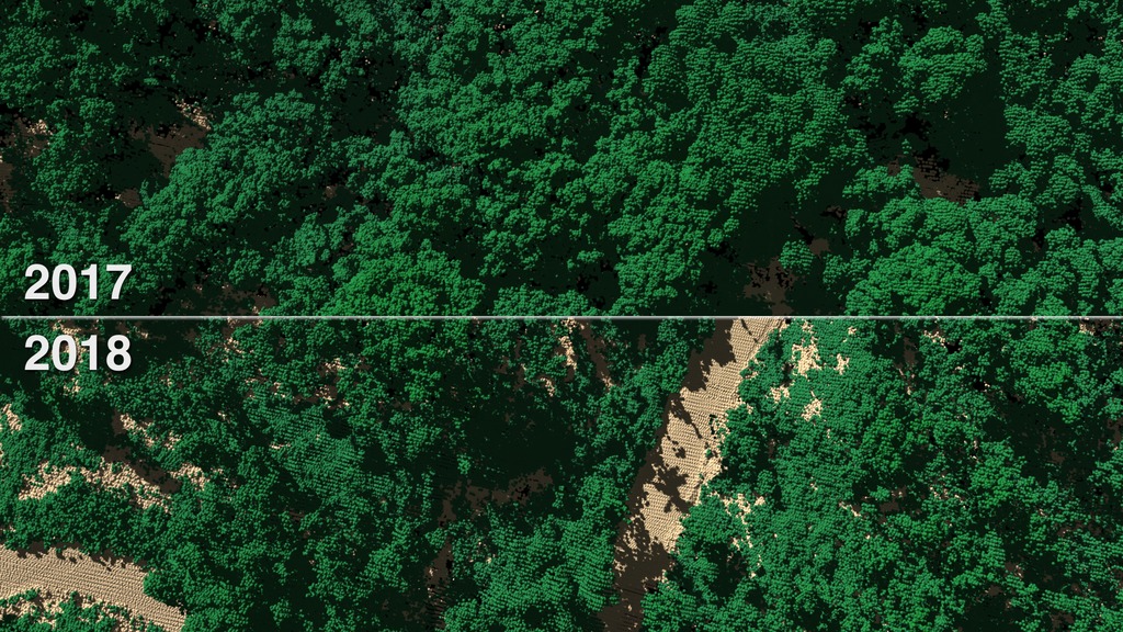
Damage to El Yunque National Forest, Puerto Rico
https://svs.gsfc.nasa.gov/4621
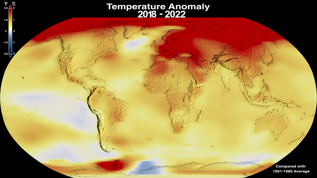
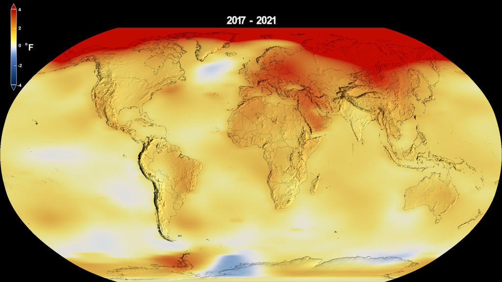
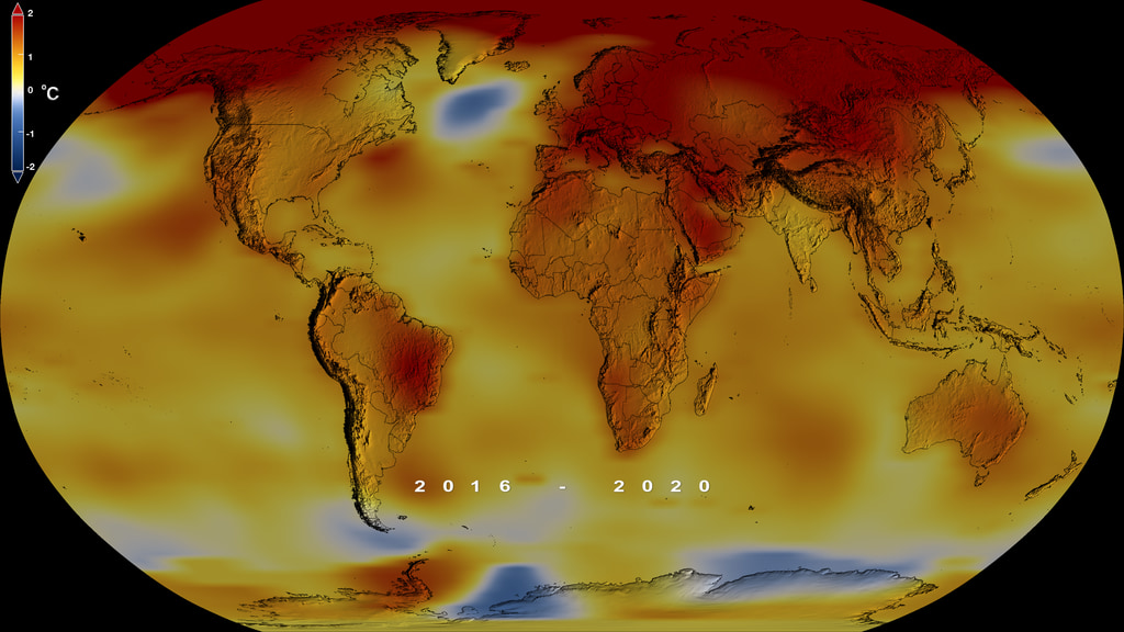
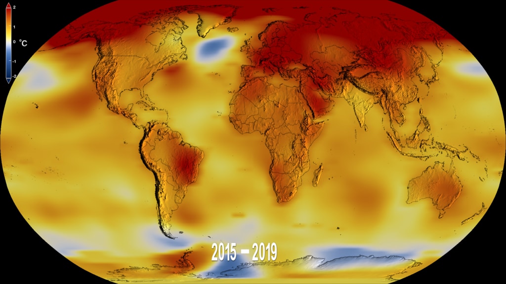
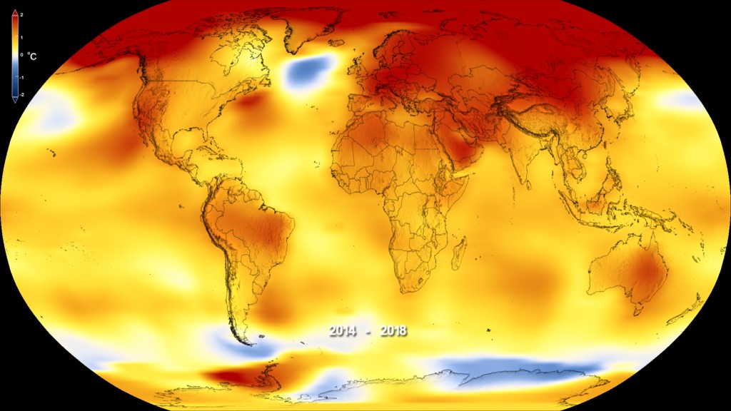
Global Temperature Anomalies from 1880 to 2018
https://svs.gsfc.nasa.gov/4626
City Lights from the International Space Station
https://earthobservatory.nasa.gov/images/92912/earth-awash-in-lights-of-the-night
Earth’s Magnetosphere
https://svs.gsfc.nasa.gov/4663
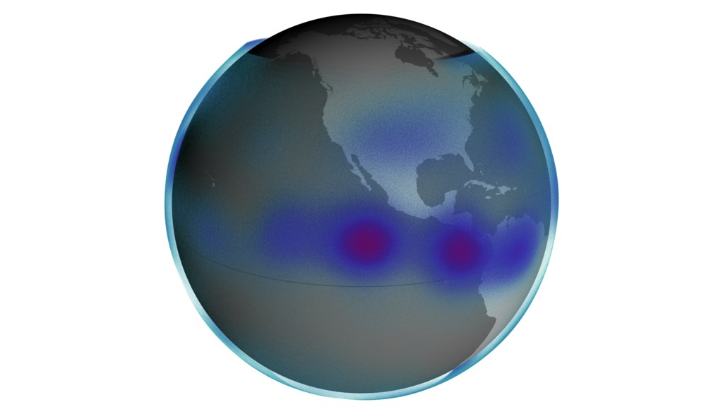
Ozonewatch 2018
https://svs.gsfc.nasa.gov/30985
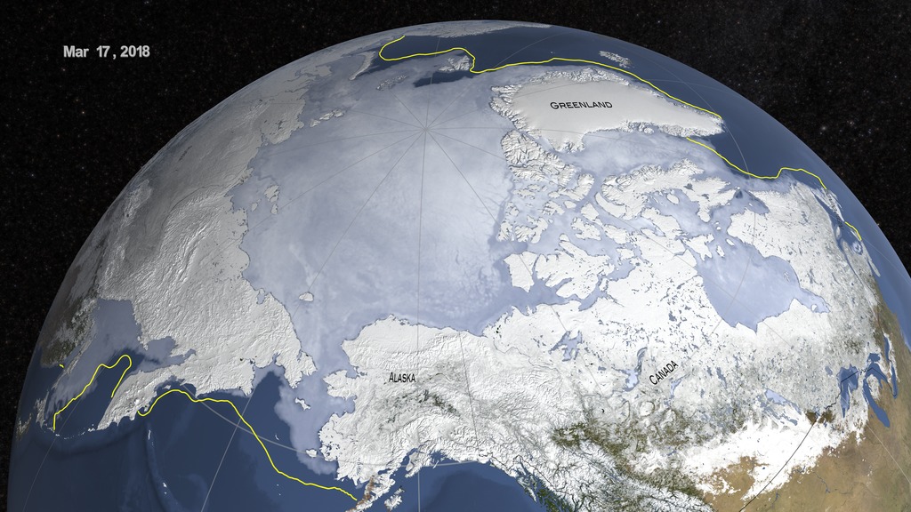
Sea Ice Maximum Extent 2018
https://svs.gsfc.nasa.gov/4628
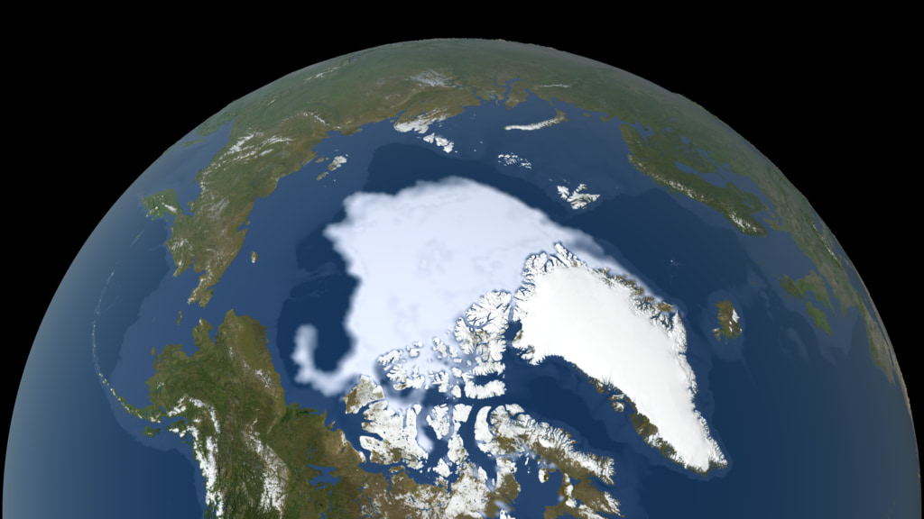
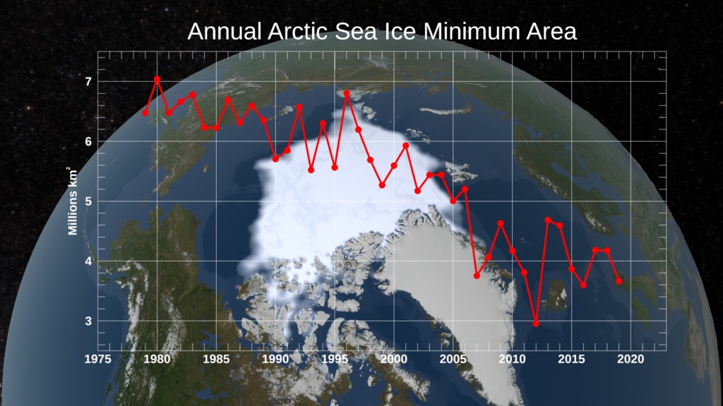
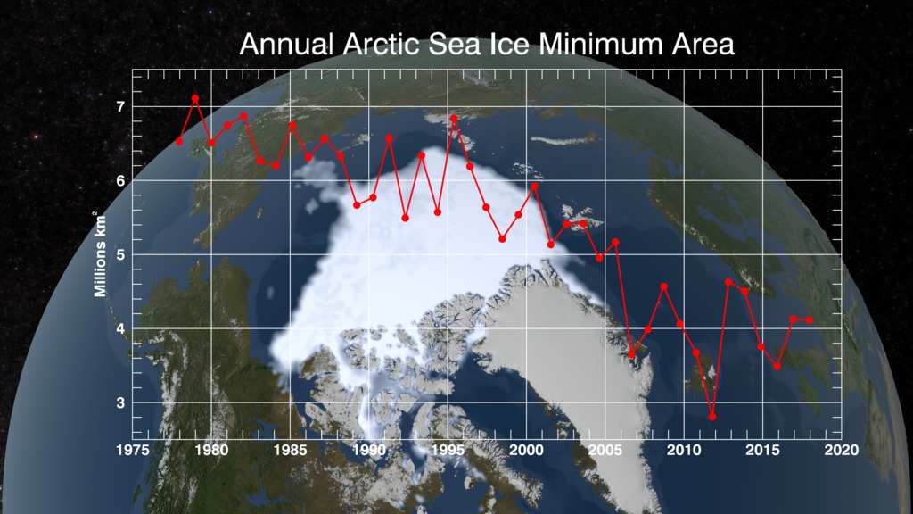
Annual Arctic Sea Ice Minimum 1979 - 2018
https://svs.gsfc.nasa.gov/4686
Average Motion of Greenland Ice Sheet
https://svs.gsfc.nasa.gov/4688
Wide View of a Shrinking Glacier: Retreat at Pine Island
https://earthobservatory.nasa.gov/features/pine-island
Changes of the Padma River
https://earthobservatory.nasa.gov/world-of-change/PadmaRiver
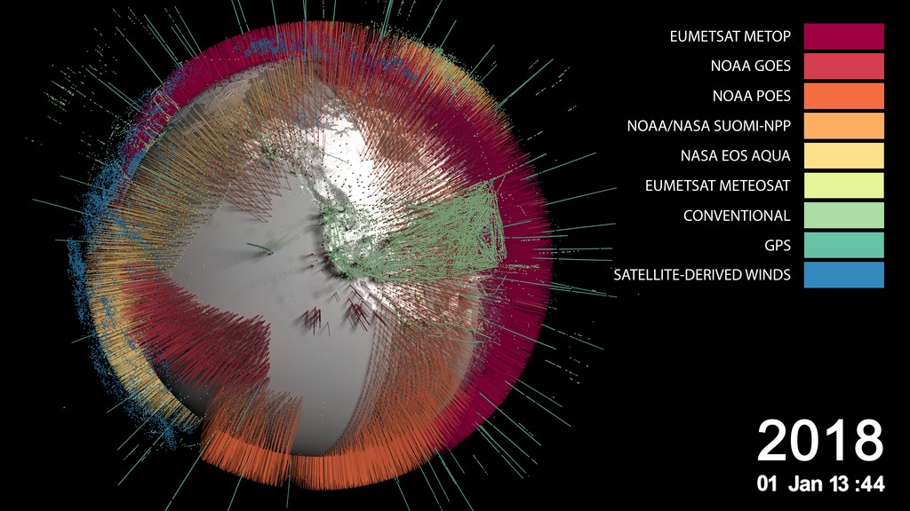
Evolution of the Meteorological Observing System
https://svs.gsfc.nasa.gov/4654
Global Fire Weather Database
https://svs.gsfc.nasa.gov/4634
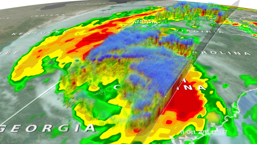
Tropical Storm Michael Drenches the Carolinas
https://svs.gsfc.nasa.gov/4692
GPM Captures Super Typhoon Mangkhut Approaching the Philippines
https://svs.gsfc.nasa.gov/4682
Ice Cube Cubesat Measures High Altitude Atmospheric Ice
https://svs.gsfc.nasa.gov/4636
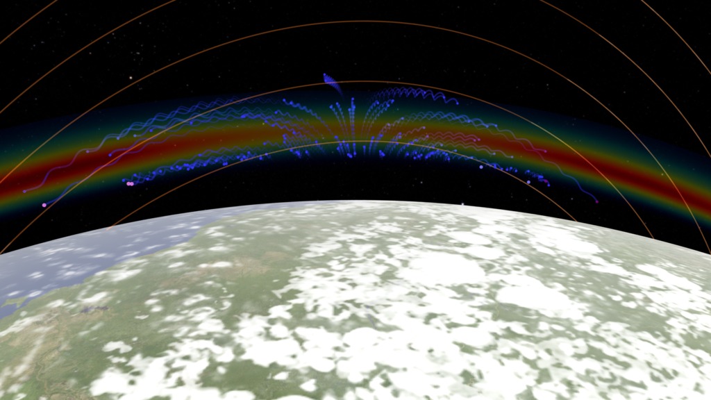
Interface to Space: The Equatorial Fountain
https://svs.gsfc.nasa.gov/4617
Midsummer Sunrise, Gulf of Saint Lawrence
https://earthobservatory.nasa.gov/images/92622/midsummer-sunrise-gulf-of-saint-lawrence
Love in the Air: Von Kármán Vortices
https://earthobservatory.nasa.gov/images/144556/love-is-in-the-air
Cloudy Congo River Basin
https://earthobservatory.nasa.gov/images/144608/cloudy-congo-river-basin
Europe at Night
https://earthobservatory.nasa.gov/features/NightLights
International Space Station: Canada at Night
https://eol.jsc.nasa.gov/BeyondThePhotography/CrewEarthObservationsVideos/
Credits
Please give credit for this item to:
NASA's Goddard Space Flight Center
-
Production assistant
- Kathryn Mersmann (USRA)
-
Producer
- Katie Jepson (USRA)
Release date
This page was originally published on Friday, April 19, 2019.
This page was last updated on Wednesday, May 3, 2023 at 1:46 PM EDT.
Series
This visualization can be found in the following series:Sources
- ID: 5060
 Visualization
 - ID: 4964
 Visualization
 - ID: 4882
 Visualization
 - ID: 4867
 Visualization
 - ID: 4787
 Visualization
 - ID: 4786
 Visualization
 - ID: 4626
 Visualization
 - ID: 4654
- ID: 4621
- ID: 4658
- ID: 4692
 Visualization
 - ID: 4686
 Visualization
 - ID: 4662
 Visualization
 - ID: 4636
 Visualization
 - ID: 4628
 Visualization
 - ID: 4617
 Visualization