Exploring Earth's Ionosphere: Limb view with approach
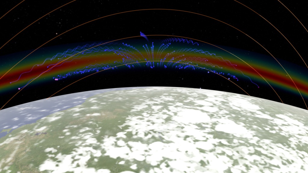
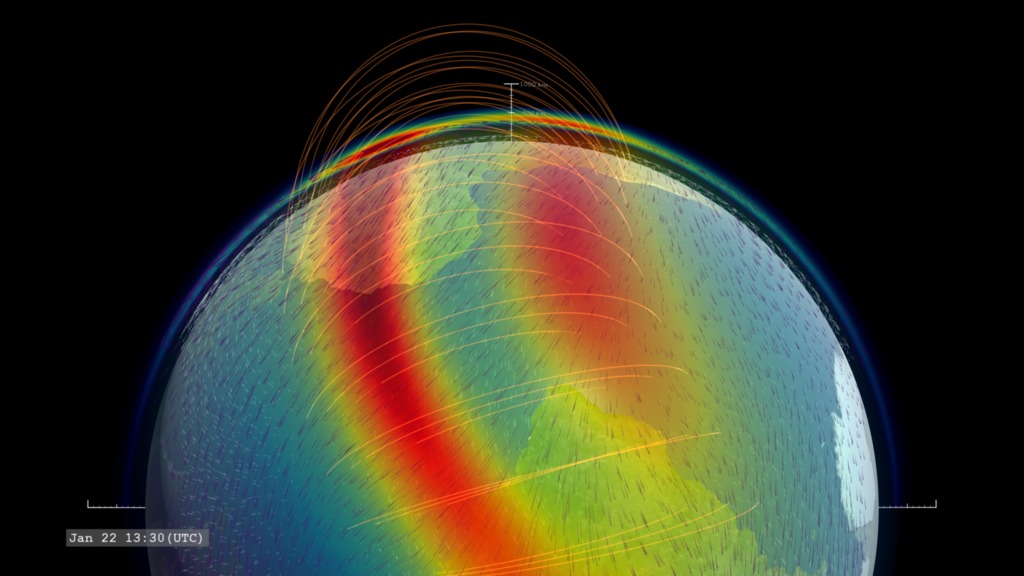
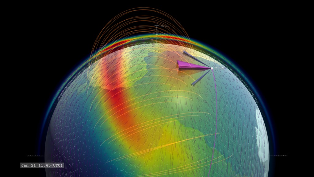
Oxygen ion enhancements at 350km altitude, ionospheric winds at altitudes of 100 km (white) and 350 km (violet) and the low-latitude geomagnetic field.
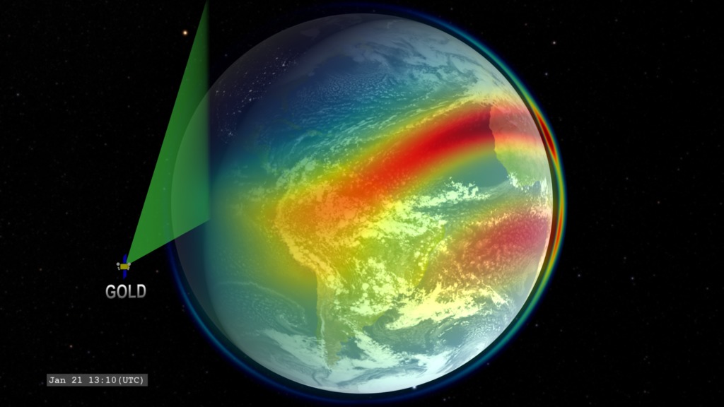
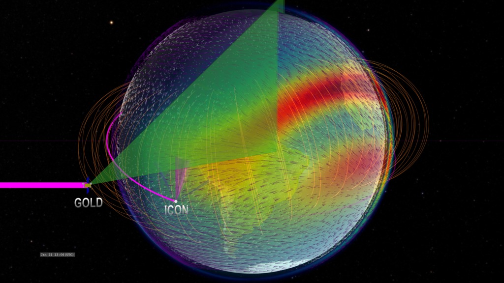
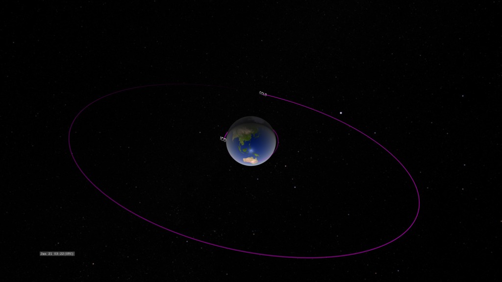
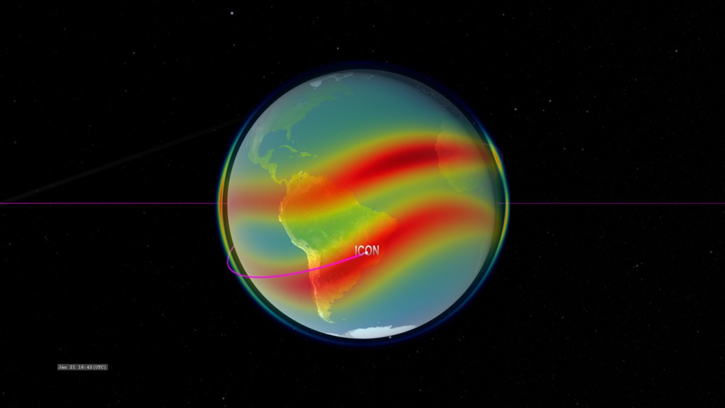
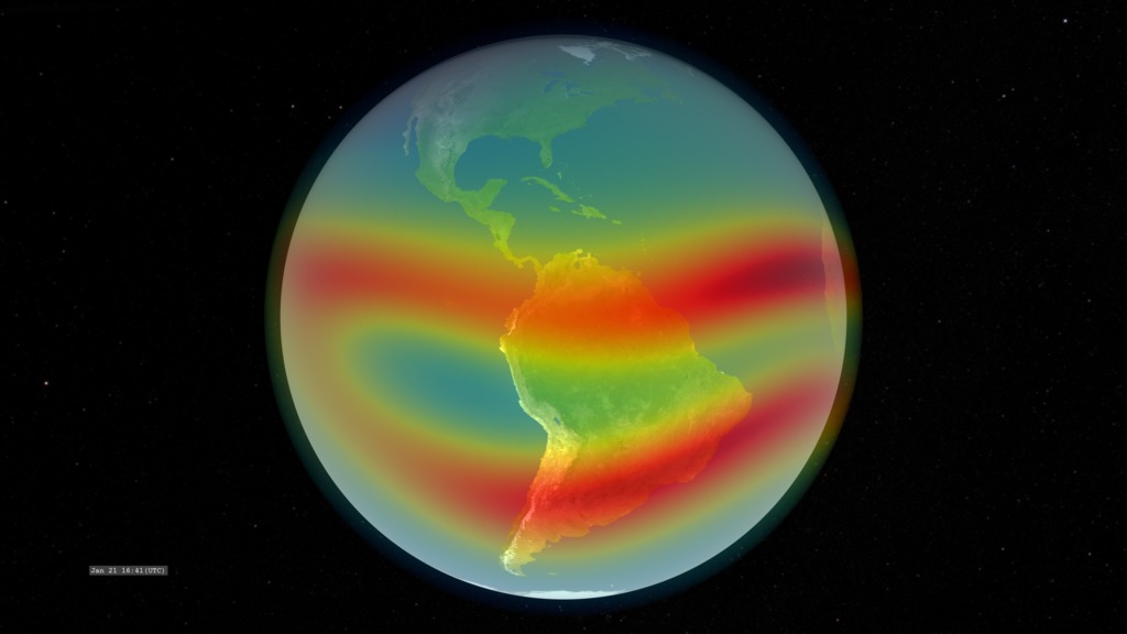
This visualization presents several 'reference models' for studying Earth's ionosphere. It opens with a full-disk view of Earth, then zooms-in to a close-up view of Earth's limb and ionospheric data-driven models, over a fixed geographic location - off the Atlantic coast of South America.
Reference models are used to define well-established knowledge and facilitate mapping out areas for future exploration. The models might be described as semi-empirical, in that they are generated using many measurements at a varietly of locations, and those measurements are used to constrain a theoretical model which is used to estimate measurements at locations where an actual measurement is not available.
Three models important in ionospheric physics are presented in this visualization.
International Reference Ionosphere (IRI)
This model provides parameters such as electron temperature and density, ion temperature and the densities of various ions (O+, H+, He+, NO+, O2+). In this visualization, we display the atomic oxygen positive ion (a single atom ion) density at an altitude of 350 kilometers. On the limb of Earth, we present a vertical cross-section of the model, illustrating how the density varies with altitude and providing an altitude scale for comparison.
This dataset exhibits two notable characteristics.
- Daily variation: The oxygen ion density increases during the day and then decreases after nightfall. This is due to photoionization by solar ultraviolet light, which increases with sunrise to a maximum at local noon, and then decreases towards evening.
- Appleton Anomaly: One of the more striking features of the ion density is the daytime enhancement is split into two regions, distributed symmetrically above and below the magnetic equator. This feature was discovered by Edward Appleton in 1946. It is now understood to be an effect of the interaction of Earth's geomagnetic field with upper atmosphere electric fields, and often referred to as the 'fountain effect,' explained in 1965. The electric fields lift ions and electrons upward by E-cross-B drift (Plasma Zoo). At higher altitudes, the upward drift decreases and the geomagnetic field and gravity dominate the motion, guiding the charged particles earthward.
Horizontal Wind Model (HWM)
This model provides speed and direction of horizontal (parallel to Earth's surface) winds constructed from over 70 million ground-based and satellite measurements. Two altitude levels are displayed in this visualization: 350 kilometers (same altitude as the IRI oxygen ion data) in violet glyphs, and 100 kilometers (white glyphs). This model only extends to 60 degrees latitude, so there are gaps around the poles in this visualization.
One of the most notable characteristics in this dataset, particularly the 350 kilometer data, is how the winds are driven by the daily solar heating cycle. As the sun rises, the upper atmosphere is heated by solar ultraviolet light. This creates a high-pressure region which drives the atmosphere away from direct sunlight; westward in the morning and eastward in the afternoon. As the sun sets and the atmosphere cools, we see the wind reverse, filling in the now cooler and lower-pressure region.
International Geomagnetic Reference Field-12 (IGRF-12)
This model provides the structure of Earth's magnetic field which is a dominant influence on the motion of electrons and ions in the ionosphere. The geomagnetic field changes very slowly over decades. For this visualization, we display only a few field lines (golden wire-like structures) near the geomagnetic equator. As we observe the daily variation of the data, particularly the oxygen ions, we see the Appleton anomaly is hedged in by the low-latitude geomagnetic field.
References
- NOAA/National Geophysical Data Center. International Geomagnetic Reference Field
- Erwan Thebault, Christopher C. Finlay, et al. International Geomagnetic Reference Field: the 12th generation. Earth, Planets and Space 67:79 (2015)
- Dieter Bilitza. The International Reference Ionosphere - Status 2013. Advances in Space Research, Volume 55, p. 1914-1927 (2015)
- Douglas P. Drob, John T. Emmert, et al. An update to the Horizontal Wind Model (HWM): The quiet time thermosphere. Earth and Space Science, vol. 2, issue 7, pp. 301-319
- Edward V. Appleton. Two Anomalies in the Ionosphere. Nature, Volume 157, pp. 691 (1946)
- E. N. Bramley and M. Peart. Diffusion and electromagnetic drift in the equatorial F2-region. Journal of Atmospheric and Terrestrial Physics, vol. 27, pp. 1201-1211 (1965)
- R.J. Moffett & W.B. Hanson. Effect of Ionization Transport on the Equatorial F-Region. Nature 206, pp705-706 (1965)
Oxygen ion enhancements at 350km altitude and the low-latitude geomagnetic field.
Oxygen ion enhancements at 350km altitude, ionospheric winds at altitudes of 100 km (white) and 350 km (violet).
Oxygen ion enhancements at 350km altitude.

Color bar for oxygen ion density.
Credits
Please give credit for this item to:
NASA's Scientific Visualization Studio
-
Visualizer
- Tom Bridgman (Global Science and Technology, Inc.)
-
Scientists
- Jeff Klenzing
- Sarah L. Jones (NASA/GSFC)
-
Producer
- Genna Duberstein (USRA)
-
Writer
- Sarah Frazier (ADNET Systems, Inc.)
-
Technical support
- Laurence Schuler (ADNET Systems, Inc.)
- Ian Jones (ADNET Systems, Inc.)
Release date
This page was originally published on Friday, January 13, 2017.
This page was last updated on Tuesday, November 14, 2023 at 12:08 AM EST.
Series
This visualization can be found in the following series:Datasets used in this visualization
-
IGRF-2012 (International Geomagnetic Reference Field)
ID: 941 -
HWM 2014 (Horizontal Wind Model)
ID: 942 -
IRI 2016 (International Reference Ionosphere)
ID: 944
Note: While we identify the data sets used in these visualizations, we do not store any further details, nor the data sets themselves on our site.
Related
- ID: 4641
- ID: 4617
 Visualization
 - ID: 12825
 Infographic
 - ID: 4610
 Visualization
 - ID: 4540
 Visualization
 - ID: 4527
 Visualization
 - ID: 4498
 Visualization
 - ID: 4503
 Visualization
 - ID: 4504
 Visualization
Alternate Versions
- ID: 4594
 Visualization
Used as a Source In
- ID: 12817
![Complete transcript available.Music credits: 'Faint Glimmer' by Andrew John Skeet [PRS], Andrew Michael Britton [PRS], David Stephen Goldsmith [PRS], 'Ocean Spirals' by Andrew John Skeet [PRS], Andrew Michael Britton [PRS], David Stephen Goldsmith [PRS] from Killer Tracks.Watch this video on the NASA Goddard YouTube channel.](/vis/a010000/a012800/a012817/GOLDOverview_YouTube.00001_print.jpg) Produced Video
Produced Video